Grooves carry the category, not the class: influence functions on VQ-tokenised CIFAR
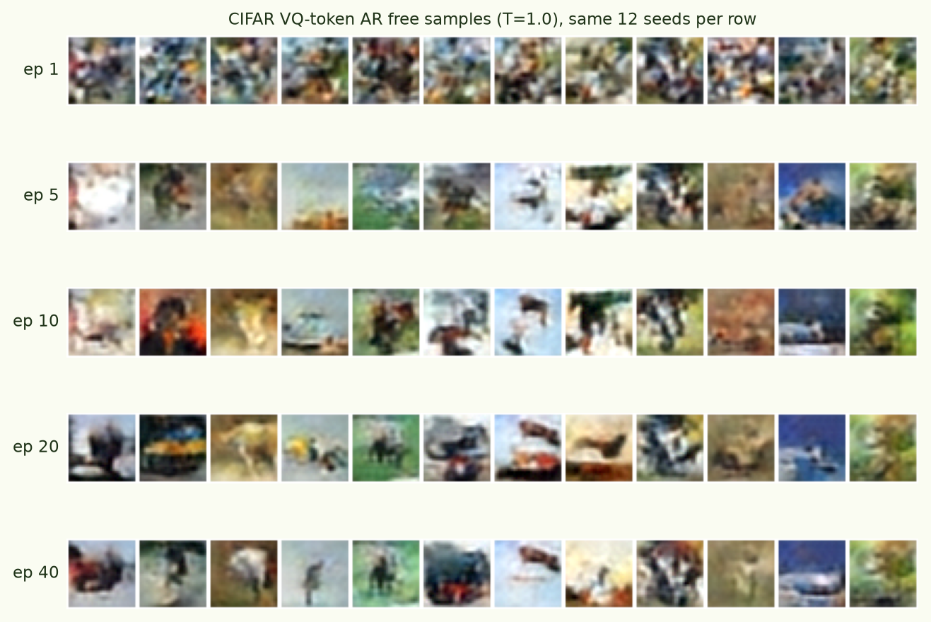
This is the scale-up of the MNIST grooves study to a real image dataset with a learned tokeniser. Each CIFAR-10 image is compressed by a small VQ-VAE into an 8×8 grid of 64 discrete codes; a decoder-only transformer models that code stream autoregressively (tied embeddings, cross-entropy — the same "language model whose language is images" recipe); and we probe its loss landscape with the same sorted estimator, gated on reproducibility. Four findings, and the third is the interesting one:
- the grooves exist and are reproducible, but are much weaker than on MNIST and — unlike MNIST — fade as training converges;
- the BIF still predicts what per-class fine-tuning does, at every checkpoint;
- unsupervised clustering recovers the coarse animate/inanimate split (animal vs vehicle) far better than pixels do — but the fine ten-class taxonomy not at all;
- the estimator story inverts: on this well-conditioned landscape the naive covariance estimator is fine, and the block-centring fix that MNIST needed is a slight net negative.
§1Setup
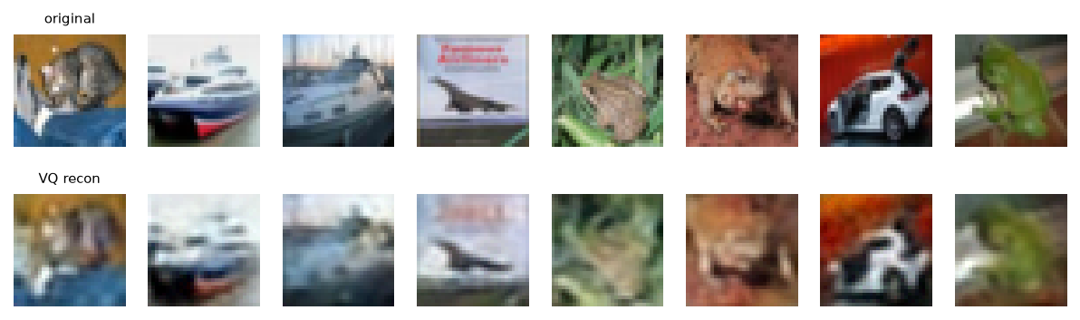
The tokeniser is a compact VQ-VAE (f=4 conv encoder/decoder, 512-entry codebook, EMA updates with dead-code restarts) trained on CIFAR's 50k images; all 512 codes stay live. Its reconstructions are blurry but class-faithful — which matters, because everything downstream sees only the codes, so whatever the VQ discards is invisible to the influence analysis.
- tokeniser
- VQ-VAE f=4, codebook 512 (512/512 live), 32×32×3 → 8×8 = 64 codes
- model
- decoder-only transformer d256 · 6 layers · 8 heads (~5M params), 64 tokens, vocab 512, tied embeddings
- training
- AdamW 3e-4, cosine, 40 epochs → 290.5 nats/image (4.54 nats/token, ≈6.55 of 9 bits/token); 1.9% train/eval gap
- BIF
- devinterp SGLD (localised, γ=100), 8 chains × 2,600 draws, ε per-checkpoint, two independent runs, gated on agreement r ≥ 0.9
- ground truth
- per-class AdamW fine-tune → ΔNLL on 510 class-balanced probes
- code & artefacts
- arcadia-impact/small-abstraction-test-{logs, mnist-ar} on HF; VQ under
cifar-vq/
§2The estimator flips: this landscape is well-conditioned
On MNIST-pixel the naive full-window covariance estimator was broken — sharp minima forced a tiny SGLD step, the chain's loss level wandered on the timescale of the whole run (a slow "common mode"), and only a block-centring high-pass rescued reproducibility. Here the opposite holds: raw covariance already reproduces at r ≈ 0.96 at every checkpoint, and block-centring is a slight net negative (~0.94). The VQ-token landscape is flat enough that the chain mixes well and there is no slow common mode to filter — so the fix that MNIST couldn't live without just discards a little signal here.
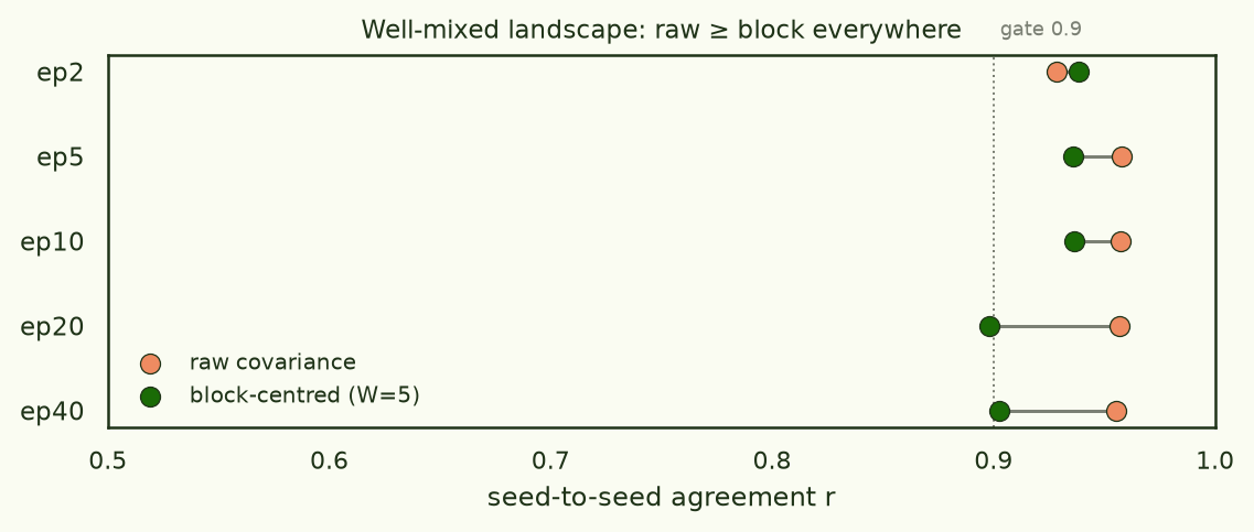
The raw-vs-block ranking is a free diagnostic of the minimum's geometry. A learned tokeniser on a real dataset gives the AR model a far better-conditioned loss landscape than raw MNIST pixels did.
§3Grooves: real, but weak and fading
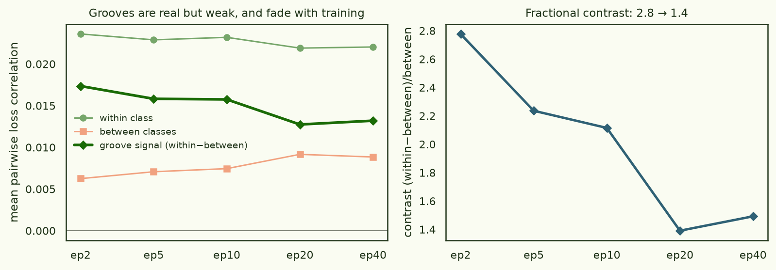
Same-class probes still co-fluctuate more than cross-class probes at every checkpoint, and every cell clears the reproducibility gate. But the effect is an order of magnitude smaller than MNIST's: within-class loss correlation sits at ~0.022 (MNIST was ~0.14), over a near-zero cross-class baseline. And where MNIST's grooves deepened toward convergence, CIFAR's fade — the fractional contrast falls from ~2.8 at epoch 2 to ~1.4 by epoch 20 and stays there.
§4Ground truth: the BIF still predicts fine-tuning
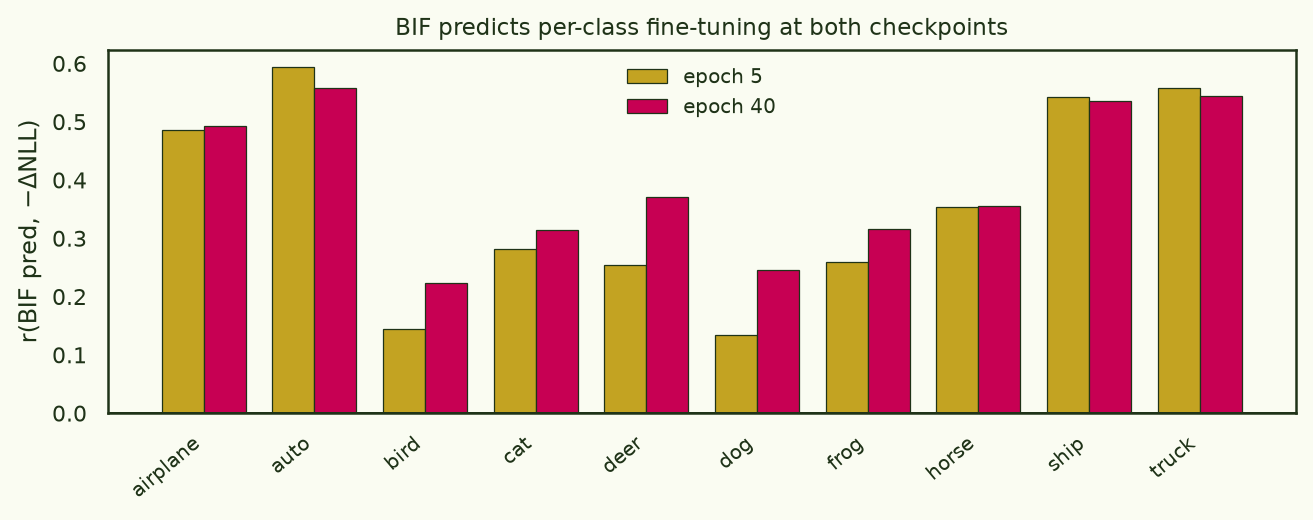
Despite the weak grooves, the influence-function reading holds: fine-tune a fresh copy on one class for 20 steps, and the BIF's class-row prediction correlates with the actual per-probe ΔNLL — mean per-class r = +0.36 at epoch 5 and +0.40 at epoch 40, sign correct 10/10 at both. So the grooves are meaningful (they predict a real behavioural effect); they just don't line up with the ten-way label taxonomy, as §5 shows.
§5The headline: the category, not the class
Now the goal — recover the abstraction without labels. Clustering the checkpoint-ensembled BIF into ten groups gives ARI ≈ 0.04 against the CIFAR classes: chance. Clustering the VQ-decoded pixels directly does no better (0.06). The fine ten-class taxonomy is simply not what this loss landscape is organised by.
But split into two clusters and ask about the superordinate animate/inanimate divide, and the BIF lands ARI ≈ 0.29 — one cluster 85% animal, the other 68% vehicle — while clustering the pixels gets only 0.09. The grooves carry the animal/vehicle abstraction three times better than appearance does, even though neither can resolve the individual classes. The loss geometry has organised the data by broad semantic category, not by the human label set.
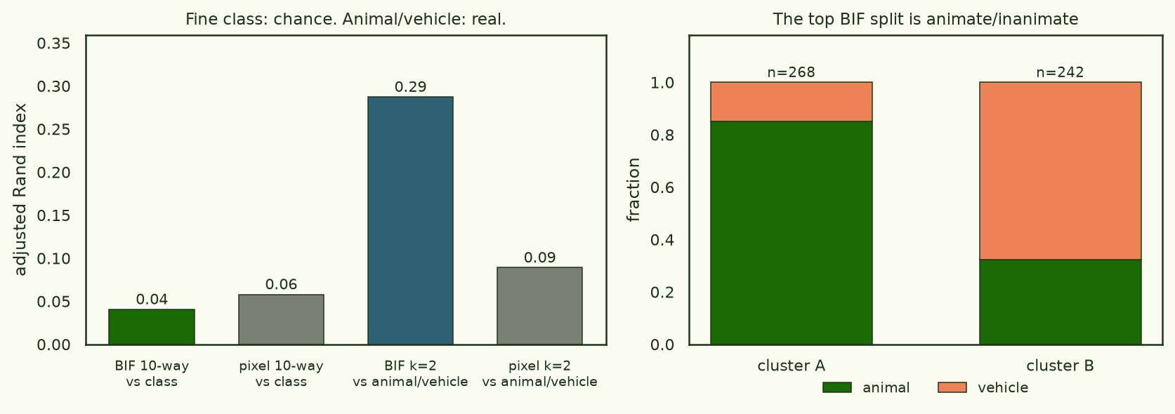
The loss-landscape grooves encode a coarse animate/inanimate abstraction that is not salient in pixel space — but not the fine ten-class taxonomy. On CIFAR the model grooves by category, not by class.
The cluster hierarchy below makes this concrete, and it's worth actually poking at. Hover any cluster to see sixteen of its member images; click to pin, click away or Esc to dismiss. The green/orange rail on each node marks animal- vs vehicle-majority. As you sweep k from 2 rightward, the top split holds its animal/vehicle character (the rails stay sorted) while the per-class colours inside the nodes stay stubbornly mixed — you can watch, image by image, that a cluster is "animals on grass" or "vehicles on grey" long before it is ever "cats" or "trucks." The ARI-vs-class under each column stays near zero throughout; the structure the eye sees in the images is categorical, not class-level.
§6What it means, and the honest limits
Two readings, and I can't fully separate them from this experiment. The optimistic one: the loss landscape encodes a genuine superordinate abstraction (animate vs inanimate) that sits above the label set, which is exactly the kind of structure the natural-abstractions hypothesis predicts should be robust — and it's more semantic than pixels, so it isn't just background colour. The deflationary one: "animal vs vehicle" still correlates with coarse scene statistics (foliage/ground vs sky/road/water), and a 512-code f=4 VQ throws away exactly the fine detail (a cat's face, a truck's wheels) that would distinguish classes within a category — so the fine-class failure may be as much the tokeniser's information loss as a fact about the landscape.
| claim | status | evidence |
|---|---|---|
| grooves exist, reproducible | yes | gated r 0.90–0.94 |
| BIF predicts fine-tuning | yes | r +0.36/+0.40, sign 20/20 |
| coarse animal/vehicle recovered | yes, > pixels | ARI 0.29 vs 0.09 |
| fine ten-class recovered | no (chance) | ARI 0.04 |
| grooves deepen with training | no — they fade | contrast 2.8 → 1.4 |
The clean next test that would separate the two readings is a better tokeniser (more codes, or f=2 for 256 tokens) rather than a bigger transformer — if fine-class structure appears once the codes preserve within-category detail, the failure was the tokeniser; if it stays coarse, the landscape genuinely grooves by category. A larger AR model is the cheaper thing to try first, but I'd expect the tokeniser to be the binding constraint here.
Artefacts · HF small-abstraction-test-logs (all SGLD traces, BIF matrices, the 40-epoch checkpoint set) · small-abstraction-test-mnist-ar (VQ tokeniser under
cifar-vq/).
Compute · 1× H100 ≈ 4.5 h ≈ $15 (tokeniser + 40-epoch train + five gated BIF cells at 8×2,600 draws + fine-tune). Pod deleted after verified upload.