What does a pretrained RandAR cluster? Colour ⊗ content in the loss landscape
Everything else in this thread trained its own small model. Here we instead take an off-the-shelf strong generator — RandAR-L (0.3B params, ImageNet-256), a transformer (Pang et al., CVPR 2025) with FID 2.65 — and probe its loss landscape with the . Two questions: (1) what does the BIF cluster ImageNet images by, and how does that change when we score only the last fraction of a random token order (each cell predicted from a large scattered context)? (2) Can the BIF similarity be factored into two independent axes — the image analogue of digit ⊗ stroke-width?
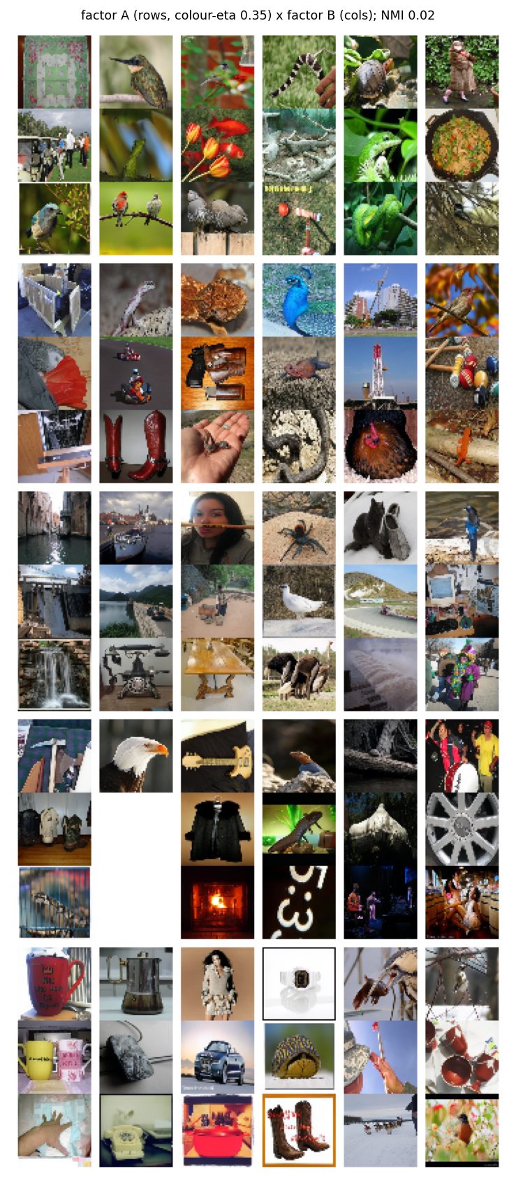
The short answer to (2), and the nicest result here: yes — the dominant factorisation is predominant colour ⊗ content.
§1Setup
- model
- pretrained RandAR-L 0.3B (ImageNet-256), random-order AR, LlamaGen VQ tokeniser (f=16, 16384 codes → 256 tokens). Loaded as-is; verified by generation.
- BIF
- localised over all 0.3B params, gradient from the model's own random-order NLL (null/unconditional class) on ImageNet-256 minibatches; 4 chains × 2 seeds, block-centred covariance.
- readouts
- per-token NLL of the tail of a random order — full · last-7/8 · last-3/4 · last-1/2 — on 500 held-out ImageNet-val images (unlabelled; clusters are unsupervised).
- reproducibility
- seed-to-seed off-diagonal agreement ≈ 0.53–0.56 — moderate: BIF on a big single checkpoint is noisier than the small-model regime, so read the clusters as real-but-soft.
- code & artefacts
- RandAR weights are public (
ziqipang/RandAR); our BIF code + matrices onarcadia-impact/small-abstraction-test-{logs}.
§2The clusters, and how they change down the order
An interactive cluster hierarchy of the 500 probes as the number of clusters grows k=2→32 (flows top→bottom). Nodes are tinted by their members' dominant colour; hover any box for a grid of its member images (click to pin, Esc to dismiss). Toggle which readout drives the clustering:
Note (2026-07-05): these fractions restrict only the loss readout — the SGLD perturbation targets the full loss, so all four share one posterior. That is not masking the fine-tuning. For the corrected experiment that masks the perturbation gradient too — and moves the clustering off colour — see Masking the fine-tuning loss.
§3Factored: predominant colour ⊗ content
Is the similarity a single axis, or a product of independent ones? We spectrally embed the BIF, take the dominant grouping (factor A), deflate it out of the embedding, and cluster the residual (factor B). The two come out nearly independent (normalised mutual information 0.02), and they split cleanly by meaning:
The content axis as its own splitting diagram
Section 3's grid shows the content factor as columns; here it is as its own interactive hierarchy. We take the full-loss BIF, remove the dominant colour factor (deflate its cluster-indicator subspace out of the spectral embedding), and cluster the residual as k grows 2→32. Hover any node for member images (click to pin, Esc to dismiss). Toggle the tint:
§4Reading this honestly
Two caveats. First, the gate is moderate (~0.55), not the ≥0.9 of the small-model studies: localised SGLD over a 0.3B pretrained model from a single checkpoint gives a noisier posterior (the chain drifts ~10–30% in loss over its length; block-centring recovers the local covariance but reproducibility is capped). The clusters and the colour⊗content factoring are stable across seeds in their gross structure, but individual assignments are soft. Second, the colour axis is partly the VQ tokeniser's doing — a code-based model necessarily encodes colour strongly — so "colour ⊗ content" is a statement about this model+tokeniser, not a universal law. Still: the factoring is a clean, independent-axes decomposition, and the content axis is real structure a pure colour histogram would miss.
Reader-requested: run the probe on a real pretrained RandAR at image scale, and try to find a factored (colour ⊗ content) cluster structure. Both done.
Model: RandAR-L 0.3B, ziqipang/RandAR (Pang et al., CVPR 2025) + LlamaGen
VQ. Code: randar_pretrained.py, randar_pretrained_bif.py,
analyze_pretrained.py, factored_cluster.py. BIF matrices + configs on
HuggingFace arcadia-impact/small-abstraction-test-logs. 1× H100.