Grooves without labels: influence functions on a class-blind STL-10 model

The CIFAR result showed the loss-landscape grooves carry a coarse animate/inanimate abstraction. But that model was trained on labelled data — could the abstraction be leaking in through the label distribution somehow? This piece removes labels entirely: a VQ-tokenised autoregressive transformer trained on STL-10's 100,000 unlabelled images at 64×64 (twice CIFAR's resolution), which never sees a single class label. We then probe it with the labelled test set purely for evaluation. Three findings:

• The abstraction is not from supervision. A completely class-blind model still carves grooves whose unsupervised clustering recovers animal-vs-vehicle at ARI ≈ 0.37 — versus ≈ 0.00 from clustering the pixels. Fine ten-class identity stays at chance.
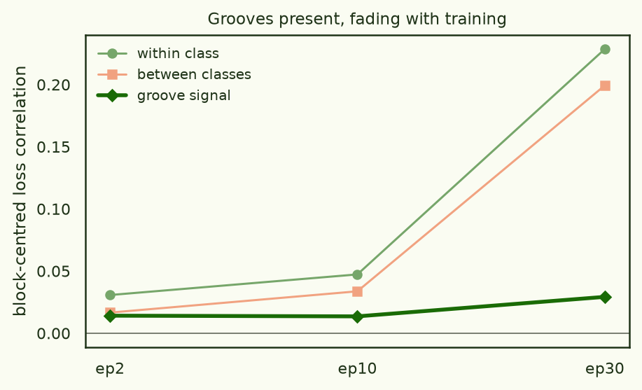
• The grooves are real but weak and fade with training, as on CIFAR.
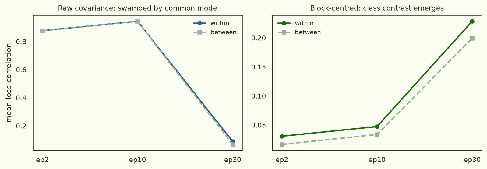
• The estimator lesson deepens: at this scale the cold checkpoints are common-mode-dominated, so the block-centred estimator (from the MNIST piece) is not optional here — the raw covariance is reproducible but structureless.

§1Setup — no labels, higher resolution

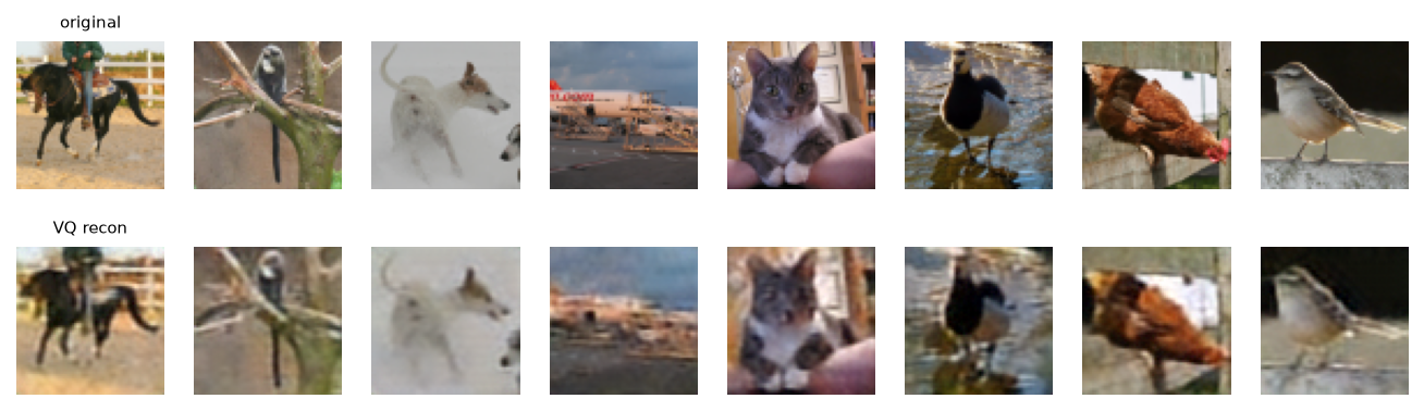
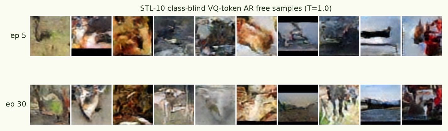
STL-10 ships a 100k-image unlabelled split precisely for unsupervised work. We train a VQ-VAE (f=4, 1024-code book) on it, giving each 64×64 image a 16×16 = 256-code grid, then train a decoder-only transformer on those code streams — the same token-AR recipe as CIFAR, just larger sequences and never a label in sight. The labelled test set (10 classes) is tokenised only to serve as evaluation probes.

§2Here the block estimator is mandatory

On CIFAR the naive covariance estimator was already fine. Not here. At the cold checkpoints (the early cells, where SGLD calibrated to a very small step) the chain wanders slowly and a global common mode dominates: every probe correlates with every other at ≈ 0.9, and within-class is indistinguishable from between-class. The raw estimator is highly reproducible (it faithfully re-measures the common mode) but carries no class signal. Block-centring — high-passing that slow mode away — is what surfaces the class contrast.

§3Grooves: present, weak, fading

With block-centring, same-class probes co-fluctuate more than cross-class at every checkpoint, and the contrast fades from training as before (block-5 fractional contrast +0.85 at epoch 2 → +0.15 at epoch 30). The absolute correlations are small, as expected for a class-blind model at higher resolution.

§4The point: a label-blind model still grooves by category

Clustering the checkpoint-ensembled block BIF: ten-way recovery is at chance (ARI ≈ 0.05), as on CIFAR. But the two-way animate/inanimate split lands at ARI ≈ 0.37 — one cluster 86% animal, the other 74% vehicle — while clustering the pixels themselves gives ≈ 0.00. And the ensemble is reproducible: two independent SGLD runs' ensemble matrices agree at r ≈ 0.93. The coarse semantic abstraction is genuinely there, recovered without labels at either training or clustering time, and it is not visible in appearance.

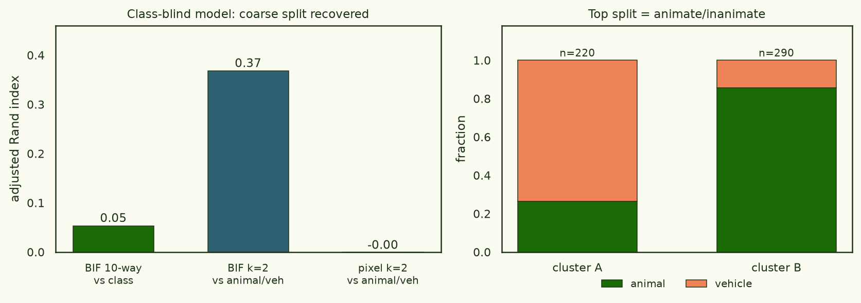
A model that never saw a label still carves a loss landscape whose grooves encode the animate/inanimate distinction — recoverable unsupervised, three-times better than from pixels. The abstraction comes from generative training alone.

The hierarchy below is interactive — hover any cluster to see its member images; click to pin, click away or Esc to dismiss. The green/orange rails mark animal- vs vehicle-majority. As k grows the top animate/inanimate split holds while the per-class colours stay mixed (fine-class ARI ≈ 0.06 throughout).

§5What it means, and the limits

This is the cleanest version of the thread's recurring finding: the animate/inanimate abstraction shows up in the loss geometry of a model trained with no labels at all, so it cannot be an artefact of label supervision — it emerges from modelling the images themselves. It is also more than surface appearance (pixels recover it at chance). The limits are the same as CIFAR's: it is a coarse abstraction, not the fine taxonomy, and a 512/1024-code VQ discards the within-category detail that would separate a cat from a dog. The natural next probe is a better tokeniser (more codes / higher resolution) to ask whether finer structure ever appears, or the product-structure question — whether the grooves factor into independent axes (identity × pose, say) rather than a single coarse partition. The next piece scales to 200 classes to push on exactly this.